Language detection using JAX
5 August 2024
Introduction
The task of language detection, in the context of deep learning, implies finding the language a word or sentence is written in. This can be done in many ways. In this article, I want to present three different approaches, gradually using more complex architectures. The first two models will be built mostly from scratch, starting with mathematics. The third and final model will be written in a more “production-ready” way, to showcase important features of the framework. Regarding the implementation framework, I’ll be using JAX.
Why JAX? I’m glad you asked! Jax is a library for composable function transformations. Its core transformations are for auto differentiation, JIT, and vectorization. Besides these features, it also enables acceleration on a GPU/TPU. It has a numpy-style API, which enables us to write linear algebra in a fast and easy way. It’s basically numpy + auto differentiation + acceleration. I want to implement these algorithms “from scratch”, but I do not want to also write the backward pass from scratch, which can be left up to JAX.
To sum it all up, three deep learning architectures (MLP, RNN, LSTM) were implemented, more or less, from scratch using JAX. We’ll be using these model to classify text into seven possible languages. The final source code is available on my GitHub: link.
Prerequisites
Before we move on to writing these models, let’s see the general structure each of these models will roughly follow: hyperparameters definition, data preparation, forward & backward passes functions, training loop, validation loss & accuracy checking, sampling, and plotting. In every source file, I have delimited these sections using numbered comments.
As I said, these models will be written in JAX. Here is a mini-tutorial for this library. JAX has a numpy-like API, as a convention we alias it as jnp when we import, after that, we can use it like numpy:
import jax
import jax.numpy as jnp

a = jnp.array([1, 2, 3])
print(a * 2) # [2 4 6]

# JAX will use a GPU by default, if you have one
print(a.devices()) # {cuda(id=0)}
Function transformations are at the core of JAX. One of the available transformations is auto differentiation:
import jax
import jax.numpy as jnp


def f(x: jax.Array) -> jax.Array:
  return (x ** 2).sum()

df = jax.grad(f)

x = jnp.array([0, 1, 2], dtype=jnp.float32)

print(f(x)) # 5.0
print(df(x)) # [0. 2. 4.]
Auto differentiation can only be applied to functions returning a scalar (think loss function). We can also change which argument to differentiate with respect to, using the argnums parameter. Let’s also check the math:
Another important transformation is JIT. By default, JAX launches each kernel operation in a function, one by one. With JIT we can compile this sequence of operations together:
@jax.jit
def f(x: jax.Array) -> jax.Array:
  x = x**2
  return x.mean()
And one more special thing about JAX: pseudo-randomness. JAX handles this in a different way from most libraries, it uses the concept of keys. A key can be created from a seed, or from another key (by splitting it). A common pattern is that we start with a base seed and a key, and we split it into a key and subkey each time we need to generate random numbers. Using the same key twice is a forbidden pattern in JAX, unless we want to generate the same numbers again.
import jax

key = jax.random.key(42)

# bad
a = jax.random.uniform(key, (3,))
b = jax.random.uniform(key, (3,))

print(a == b) # [ True  True  True]

# good
key, subkey = jax.random.split(key)
a = jax.random.uniform(key, (3,))
b = jax.random.uniform(subkey, (3,))
These are the basics of JAX! There is more to this library, but it’s enough to start building these models. You can read more about JAX here.
Dataset
To train a neural network, we need some data. A great place to find good datasets is Kaggle. I decided to use this data. It has 17 total languages, but we’ll use only 7 of them (only ascii languages). I also wrote a couple of utility functions to clear this dataset, by removing non-alphanumeric characters. You can find these functions in the data_utils.py file from the project repository.
More interesting than data cleanup is data encoding! How can we encode this data so we can efficinely later forward it through a neural network? Let’s start with a one-hot encoding for each character. A one-hot vector is full of zeros, except for one element which is one. We can have each character be a vector of the size of the vocabullary, 28 in our case, and flip the element of the correct index to one. Example:
char.shape = (vocab_size) = (28)
Let’s go one dimension deeper, a word is just a vector of characters. This yields a vector with two dimensions, each element being a one-hot vector:
word.shape = (max_chars, vocab_size) = (10, 28)
And a sentence is a vector of words. This translates to a three dimensional tensor, each element being a word. Later when we train, we will add a fourth dimension to represent the batch dimension.
sentence.shape = (max_words, max_chars, vocab_size) = (15, 10, 28)
For best practices, let’s create a train/validation dataset split:
data = get_data_params()
X, Y = get_seq_dataset(seed)

n = int(0.8 * data["data_size_seq"])

# X.shape = (5800, 15, 10, 28) -> each batch has a sentence with a max of 15 words, each has at most 10 characters
# Y.shape = (5800,) -> the correct class index for each batch

Xtr, Ytr = X[:n], Y[:n]
Xval, Yval = X[n:], Y[n:]
Similarly, we can create tensors for the model that requires a fixed size of inputs (the MLP):
X, Y = get_dataset(seed)

# X.shape = (71416, 10, 28) -> each batch has a word with at most 10 characters
# Y.shape = (71416,) -> the correct class index for each batch
# the rest is the same
Check the repository for the full source code, there are more tiny boring details, such as data padding. After all of this work, we can finally go into the neural network models! :)
MLP
The first model we are going to build is a Multilayer perceptron. It’s a network based on linear regression, however it adds activation functions between layers for nonlinearity. This adds more flexibility to the model and enables better pattern recognition. If we didn’t have activation functions, or we used the identity function as an activation, it can be mathematically proven that multiple of those layers can be equivalent to one layer with one weight matrix and a bias. We are going to have 2 layers, with a tanh activation function between. The following formula can describe our model:
Y hat denotes are prediction. The first layers is feed in as input to the tanh. The output of the activation function is the input for the second and final layer, which will output our prediction, also known as logits. We need to define the parameters of the network. It’ll have one linear hidden layer and one linear output layer. A linear/dense layer implies a weights matrix and a bias vector. This means our network will require four parameters, which I will also put in a list so it will be easier later to update the parameters.
n_input = data["vocab_size"] * data["max_chars_in_word"]  # 28 * 10
n_hidden = 100
n_output = data["num_classes"]  # 7

W1 = jax.random.uniform(key, (n_input, n_hidden)) * 0.05  # kaiming init
b1 = jnp.zeros((n_hidden))
W2 = jax.random.uniform(key, (n_hidden, n_output)) * 0.01
b2 = jnp.zeros((n_output))
parameters = [W1, b1, W2, b2]
The forward pass takes in the model parameters and an input array X. It’s a common idiom in JAX to have an immutable model architecture/module and to pass the mutable parameters around, which we’ll better see with later models when we’ll also use Flax and Optax. In this simple example, the model parameters can be represented as a list of JAX arrays. First, we need to reshape the input so we can multiply it with the weights. The zip method in Python takes two iterators and binds them together, thus we can iterate over the parameters with Ws and bs for each layer at a time. This of course requires attention when declarating the parameters array. It will become clearer in later models, once we introduce PyTree as a better abstraction for models.
@jax.jit
def forward(params: list[jax.Array], X: jax.Array) -> jax.Array:
  # from (batch, 10, 28) to (batch, 280)
  h = X.reshape(-1, n_input)

  # go until the layer before the last one
  for W, b in zip(params[:-2], params[1:-2]):
    # hidden layer
    hpreact = h @ W + b
    h = jnp.tanh(hpreact)

  # output layer
  logits = h @ params[-2] + params[-1]
  return logits
To measure how well our model is going, we are going to use the cross entropy loss function. It’s a common loss function for classification tasks. It’s also equivalent to measuring the negative log likelihood of the softmax of the logits. Here is a naive implementation in code:
@jax.jit
def get_loss(params: list[jax.Array], X: jax.Array, y: jax.Array):
  logits = forward(params, X) # y hat

  # cross entropy loss
  counts = jnp.exp(logits)
  prob = counts / counts.sum(1, keepdims=True)
  loss = -jnp.mean(jnp.log(prob[jnp.arange(y.shape[0]), y]))

  return loss
Here we are adding a JIT transformation to speed up the execution of the function. Notice we are taking in the parameters of the model and we compute the forward pass inside. This is a common JAX idiom. Thanks to this, we can create a get_grad function, which applies the auto differentiation transform to the loss function, it will differentiate with respect to the first argument (the model parameters) by default.
# differentiate with respect to the first argument (model params)
get_grad = jax.grad(get_loss)


@jax.jit
def update(params: jax.Array, gradient: jax.Array) -> jax.Array:
  # stochastic gradient descent
  return [p - lr * grad for p, grad in zip(params, gradient)]
Now we have the three main puzzle pieces that define our neural network: model parameters, a forward pass, and a backward pass. The forward pass will propagate the input through the network until we get a final vector of probabilities, which should predict the correct label (the language the text passed in is written in). The backward pass first will differentiate the loss function with respect to the model parameter, and then it will update the parameters with the specific gradient multiplied by a learning rate, set as a hyperparameter. Putting all of these togheter, we can write a training loop:
for step in range(steps + 1):
  # mini-batch
  key, _ = jax.random.split(key)  # get a new key from jax
  ix = jax.random.randint(key, (batch_size,), 0, Xtr.shape[0])
  Xb, Yb = Xtr[ix], Ytr[ix]

  # forward pass
  loss = get_loss(parameters, Xb, Yb)
  lossi.append(loss) # for the plot

  if step % 500 == 0:
    print(f"step {step}: loss={loss:.2f}")

  # learning rate decay
  if step == decay_step:
    lr /= 10

  # backward pass
  gradient = get_grad(parameters, Xb, Yb)
  parameters = update(parameters, gradient)
We use mini-batches to speed up our training loop. First we choose a mini-batch, run it through the forward pass, get the loss and after that comes the backward pass. In JAX, we could also run only the backward pass, since JAX doesn’t require us to run the function normally before differentiation, we could also just mark the get_loss function as jax.grad and it would also work. I’m writing code this way to better show the elements of the training loop.
Well, after we let the training loop run for about 20k steps, we can get quite a decent model. I managed to get a 66.72% accuracy with a 0.96 validation loss. These values will improves with more advanced models, but for the moment it works. Here is how to compute the validation loss. (spoiler: very easy!)
valid_loss = get_loss(parameters, Xval, Yval)
print(f"valid_loss={valid_loss:.3f}")  # best loss is 0.969
We can also sample from the model to test how well it works in practice. It prooves to work quite well on simple & common words. Besides this implementation, we could also ask the user for input and predict that. JAX also provides a function jax.nn.softmax which would simplify this code (and work much faster as a single kernel on the GPU), but I left the explicit implementation for now.
words = ["hola", "energy", "nicht", "ciao", "haben", "ich"]
# preds: spanish, english, german, italian, german, german
for word in words:
  enc = encode_word(word)
  logits = forward(parameters, enc)[0]

  # softmax
  counts = jnp.exp(logits)
  prob = counts / counts.sum(0, keepdims=True)
  label_index = jnp.argmax(prob, 0)
  print(f"{word}: {data['labels'][label_index]}")
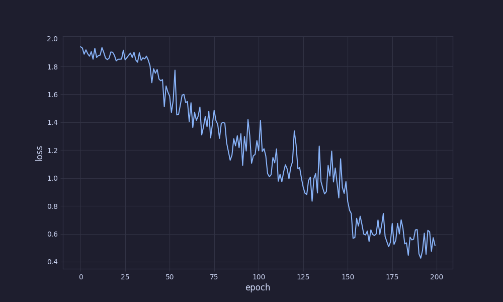
Remember we added our loss to a list? We can use that to plot it now. As a note, I used kaiming initialization for model parameters so we get a better loss in the beginning, thus helping our model to learn faster.

This concludes our MLP module. It’s the foundation for the later models. The training loop, backward pass, and loss function will be basically the same for the following networks. The model architecture and parameters will provide essential improvement.
RNN
Recurrent neural networks allow for variable-sized input. Thanks to their temporal structure, RNNs can learn patterns from sequences. Instead of feeding in a single word, we will feed in a sequence of words (a sentence). RNNs achieve this using a hidden state, which is fed in for every word. It is modified by a hidden layer, used to encode special temporal information.
The t in the upper side of the variables indicates the time step. As you can see, the first linear layer maps the input to the hidden state. The second hidden layer maps the hidden state to itself. These two layers are summed up together, which is why we need a single bias. The output of this sum is the input for the tanh activation function. The final layer takes the hidden output and maps it to the output logits.
This approach is great for encoding temporal information, however it has two main flaws. Its linear nature requires inputs to be fed in order, which is bad for parallelism and speed. Besides this, the hidden state has a limited size, which makes it hard to encode relevant information for large sequences. We may think that the most important information can be found at a later stage in the sequence, however, an RNN will pack the whole sequence in the hidden state. The second issue can be solved by using an LSTM or GRU model. The first issue is addressed by Transformer models thanks to their attention mechanism.
For the actual implementation, I’m going to use the Equinox library. It’s a JAX library that handles utility functions to use with JAX, such as PyTree manipulation. For example, we want to use JAX auto differentiation, however, for a clean implementation, we also want the model parameters to be part of a class. PyTree is a data structure that JAX understands and can work with. Equinox enables our class to inherit PyTree structure.
import equinox as eqx

class RNN(eqx.Module):
  # jax will differentiate only floating point terms, ignoring int members
  n_input: int

  Wi2h: jax.Array
  Wh2h: jax.Array
  bh: jax.Array
  Wh2o: jax.Array
  bo: jax.Array

  def __init__(self, n_input: int, n_hidden: int, n_output: int):
    self.n_input = n_input

    self.Wi2h = jax.random.normal(key, (n_input, n_hidden)) * 0.05  # kaiming init
    self.Wh2h = jax.random.normal(key, (n_hidden, n_hidden)) * 0.01
    self.bh = jnp.zeros((n_hidden))
    self.Wh2o = jax.random.normal(key, (n_hidden, n_output)) * 0.01
    self.bo = jnp.zeros((n_output))

  def __call__(self, X: jax.Array, hidden: jax.Array) -> tuple[jax.Array, jax.Array]:
    X = X.reshape(-1, self.n_input)

    # first two layers: input to hidden and hidden to hidden
    hpreact = X @ self.Wi2h + hidden @ self.Wh2h + self.bh
    hidden = jnp.tanh(hpreact)

    # map hidden to the output logits
    out = hidden @ self.Wh2o + self.bo

    # also return the hidden state, will be used for the next
    # element in the sequence
    return out, hidden


# create the model
model = RNN(n_input, n_hidden, n_output)
For the forward pass, we need to feed the model each word from the sequence one by one along with the hidden state from the previous state. At the start, the hidden state is made only of zeros.
@eqx.filter_jit
def forward(model: eqx.Module, X: jax.Array) -> jax.Array:
  hidden = jnp.zeros((1, n_hidden))

  for i in range(X.shape[0]):
    logits, hidden = model(X[i], hidden)

  return logits
We also annotate the loss function with filter_value_and_grad from Equinox. This way it returns a tuple, the first value being the actual value and the second value being the gradient. This is just another way to achieve the same thing but with only one function call.
@eqx.filter_value_and_grad
def get_loss(model: eqx.Module, X: jax.Array, y: jax.Array):
  logits = forward(model, X)

  # cross entropy loss
  counts = jnp.exp(logits)
  prob = counts / counts.sum(1, keepdims=True)
  loss = -jnp.mean(jnp.log(prob[0, y]))

  return loss
The training loop is essentially the same. Running it for 20k steps with learning rate decay and SGD update yields better results than the MLP.
In the end, we get an accuracy of 80.17% with a validation loss of 0.61. Check out the GitHub repository for the full source code.
LSTM
The last but not least model we’re going to try is the Long short-term memory (LSTM). LSTMs solve the issue of encoding and remembering useful information by utilizing gates: the input, forget, cell and output gates. These gates control how much information is allowed to flow into and out of the cell. We won’t implement these from scratch, since it requires a little more effort and code, while only being an optimization already overkill for this toy project.
To also introduce more JAX concepts, I decided to use the Flax and Optax libraries. Flax is a library that offers neural network utilities and modules to more easily compose models in a functional way. A flax model is immutable, so we need to initialize its parameters separately. Optax is a library for gradient optimization, which implements common industry standard algorithms such as Adam, which we are going to use to improve our results. Here is our model class definition, deriving from the Flax Module base class.
from flax import linen as nn
from flax.training import train_state
import optax

class LSTM(nn.Module):
  sentence_size: int
  input_size: int
  hidden_size: int
  output_size: int

  def setup(self):
    self.lstm = nn.OptimizedLSTMCell(features=self.hidden_size)
    self.h2o = nn.Dense(self.output_size)

  def __call__(self, x):
    x = x.reshape(-1, self.sentence_size, self.input_size)
    batch_size, seq_length = x.shape[0], x.shape[1]
    carry = self.lstm.initialize_carry(
      key, (batch_size,))

    outputs = []
    for t in range(seq_length):
      carry, y = self.lstm(carry, x[:, t])
      outputs.append(y)

    output = outputs[-1]
    output = self.h2o(output)

    return output
To actually create the model we need to initialize its parameters in a varibale. For this we need to feed in an example input, so Flax can figure out the shapes. After we create the model and its parameters, we can create an Adam optimizer and initialize a train state. A train state is a useful utility that helps manage state related to the training process.
nput_size = data["max_chars_in_word"] * data["vocab_size"]
hidden_size = 128
output_size = data["num_classes"]

# initialize the model
model = LSTM(sentence_size=data["max_words_in_sentence"], input_size=input_size, hidden_size=hidden_size,
             output_size=output_size)

# create an example input to initialize the model parameters
ix = jax.random.randint(key, (batch_size,), 0, len(Xtr))
example_input = Xtr[ix]

# initialize model parameters
variables = model.init(key, example_input)
params = variables['params']

# define a simple optimizer and training state
optimizer = optax.adam(learning_rate=lr)
state = train_state.TrainState.create(
  apply_fn=model.apply, params=params, tx=optimizer)
The loss function is very similar, however it uses Flax functions to achieve better performance. We also use optax to update the parameters in the backward pass.
@jax.jit
def compute_loss(params, batch, targets):
  logits = model.apply({'params': params}, batch)
  one_hot_targets = jax.nn.one_hot(targets, num_classes=output_size)
  loss = optax.softmax_cross_entropy(logits, one_hot_targets).mean()
  return loss


@jax.jit
def train_step(state, batch, targets):
  def loss_fn(params):
    return compute_loss(params, batch, targets)
  grad_fn = jax.value_and_grad(loss_fn)
  loss, grads = grad_fn(state.params)
  state = state.apply_gradients(grads=grads)
  return state, loss
The training code is much shorter this time. We update the train state each step, it holds the parameters and the method to update them using the optimizer.
for step in range(steps + 1):
  key, _ = jax.random.split(key)
  ix = jax.random.randint(key, (batch_size,), 0, len(Xtr))
  Xb, Yb = Xtr[ix], Ytr[ix]

  state, loss = train_step(state, Xb, Yb)
  lossi.append(loss)

  if step % 500 == 0:
    print(f"step {step}: loss={loss:.2f}")

On a side note, this is definitely overfitting. To take advantage of an LSTM model, we would need a larger or more complex dataset. However, we are getting good results with a final 95.27% accuracy and a 0.27 validation loss.
Conclusion
Language classification can be challenging task, however, with modern deep-learning algorithms it can be tackled in a matter of hours. We looked at three different neural network architectures, each improving on the previous one. JAX is a powerful functional library that enables fast calculations, however it can take time to get used to it. Personally I like to use JAX when I want to implement something “from scratch”, without a manual backward pass. I have also written PyTorch versions of these models in the repository, so you can compare the code and implementation differences.
References
- “The Unreasonable Effectiveness of Recurrent Neural Networks”: https://karpathy.github.io/2015/05/21/rnn-effectiveness/
- “Language modeling with Jax and RNNs”: https://svenschmit.com/jax-language-model-rnn
- JAX docs: https://jax.readthedocs.io/en/latest/quickstart.html
- Flax docs: https://flax.readthedocs.io/en/latest/
- Optax docs: https://optax.readthedocs.io/en/latest/
- Equinox docs: https://docs.kidger.site/equinox/examples/train_rnn/
- Pytorch docs on LSTM: https://pytorch.org/docs/stable/generated/torch.nn.LSTM.html