Most JPEG restoration models are built like image generators: big, expensive, and happiest when they have time to think. I wanted the opposite — something small enough to run on a single consumer GPU, fast enough to process HD video in real time, and still good enough to actually remove block artifacts instead of smearing them.
Deterministic vs. generative restoration
There are two broad ways to attack artifact removal. The deterministic route, things like SwinIR, trains a regression model with pixel-level losses such as MSE or MAE. These models are fast and cheap — often one forward pass — but they optimize for the average of many plausible clean images, which produces blurry, overly smooth results. Fine textures get washed out and the output can look worse than the original compression, just in a different way.
Generative restoration, on the other hand, models a distribution of plausible clean images conditioned on the compressed input. It can keep sharp details, produce textures humans prefer, and hallucinate sensible structure where the JPEG has destroyed information. The usual cost is speed: diffusion and flow models need tens or hundreds of network evaluations.
This project sits in the middle. It is a generative model, trained with a flow objective and perceptual loss, so it outputs sharp, human-preferred details. But it is also a true one-step model at inference — no iterative solver, no distillation, no large teacher. At QF 10 and QF 20 it gets the lowest LPIPS on LIVE-1, Urban100, and DIV2K-val among the efficient methods I compared against.
The architecture is deliberately simple: an exactly invertible two-level Haar wavelet transform replaces the learned VAE, and a compact rank-enhanced linear-attention DiT predicts a clean residual. The interesting part is the training objective — conditional pixel MeanFlow — which makes one-step generative restoration possible.
One-step generative restoration with MeanFlow
Standard rectified flow learns an instantaneous velocity and then integrates it with many Euler or Heun steps. That works, but every step costs a full forward pass. MeanFlow instead works by predicting the velocity at a single instant, it predicts the average velocity over an interval, so the whole interval can be crossed in one update. That is what enables true one-step generative image restoration without distillation.
We use the convention for data and for noise. Given a clean image and noise , the conditional flow path and its velocity are
Rectified flow regresses directly and integrates it numerically. MeanFlow instead learns the average velocity over an interval :
so the whole interval is traversed by the single update
The key identity comes from differentiating with respect to :
This lets improved MeanFlow train an average-velocity predictor while still regressing onto the instantaneous velocity target, which stabilizes training without needing a teacher.
We parameterize the network as a direct clean-image predictor. It sees the noisy wavelet residual , the compressed observation , and the interval length , and outputs a clean residual estimate
The average velocity is then
At inference we just apply
once and decode the result. One update gives the headline throughput; a second update is available when you want the best LPIPS. There is no teacher model, no distillation stage, and no iterative ODE solver at inference time.
Results
The model is evaluated on full images from LIVE-1, Urban100, and DIV2K-val at JPEG quality factors 5, 10, and 20. The input QF is used only to synthesize the compressed image; the network itself estimates degradation severity internally and receives only the decoded RGB.
LPIPS
The table below compares our two-update MeanFlow checkpoint against SODiff, the strongest competitor. At QF 10 and QF 20 we achieve the lowest LPIPS across all three datasets. The margins are largest at QF 20, where compression artifacts are still recoverable.
| Dataset | QF 10 | QF 20 | ||
|---|---|---|---|---|
| SODiff | Ours | SODiff | Ours | |
| LIVE-1 | 0.1605 | 0.1599 | 0.1237 | 0.0917 |
| Urban100 | 0.1098 | 0.1027 | 0.0846 | 0.0538 |
| DIV2K-val | 0.1732 | 0.1695 | 0.1295 | 0.0995 |
To be fair, SODiff is built on Stable Diffusion 2.1 and carries far more texture and semantic knowledge, so it still leads on DISTS, MUSIQ, MANIQA, and LPIPS at QF 5. The advantage of this model is that it gets close on LPIPS at moderate compression while being roughly smaller and faster on a single consumer GPU.
Efficiency
The full system runs at 8.05 images/s at on a single RTX 3090 with two MeanFlow updates. The one-step HD variant reaches 20 images/s at 1280×720. The model has 65.32M parameters — about fewer than SODiff and fewer than SUPIR — with no VAE encoder-decoder and no text encoder.
| Method | Params (M) | NFE | Latency (s) | Throughput (img/s) |
|---|---|---|---|---|
| FBCNN | 70.10 | 1 | 0.275 | 3.63 |
| JDEC | 38.90 | 1 | 0.860 | 1.16 |
| SODiff | 1288 | 1 | 0.610 | 1.64 |
| Ours (two-update) | 65.32 | 2 | 0.1242 | 8.05 |
Qualitative comparison
Below are two crops from LIVE-1. The first pair is at QF 5; the second is at QF 10. In both cases the left image is the compressed input and the right is the one-step restoration.
The parrots show blockiness around the feathers and background foliage being reduced while the fine stripe patterns on the faces are preserved. The bikes show spoke and dirt texture coming back without the smeared look typical of regression models.
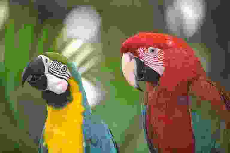
JPEG input (QF 5)
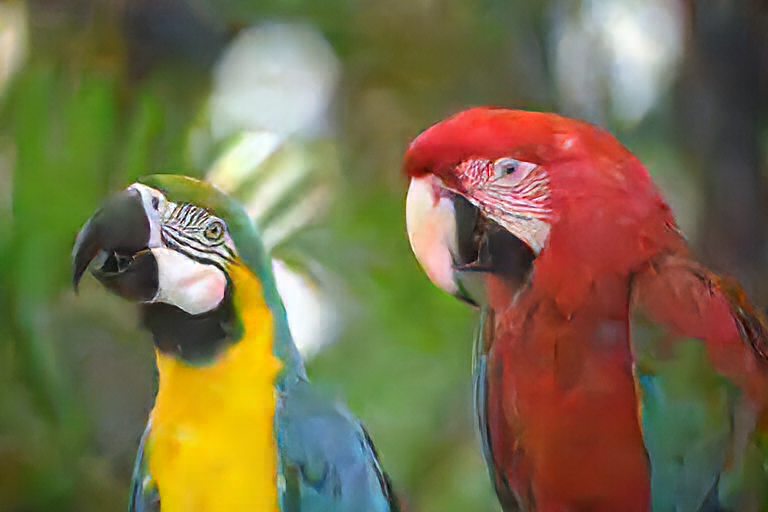
Restored (1 step)
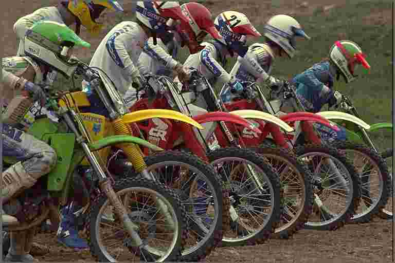
JPEG input (QF 10)
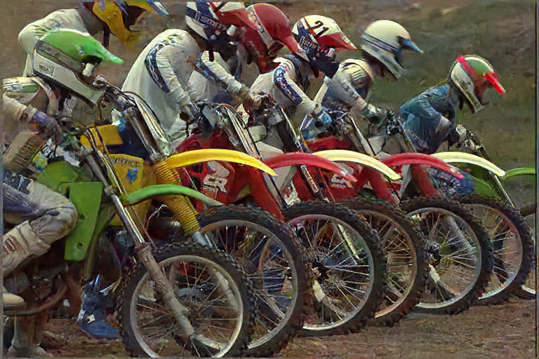
Restored (1 step)
Training on a single 3090
Everything was trained on one RTX 3090. Logging went through Weights & Biases, and I used TorchAO to experiment with quantization and other runtime optimizations once the checkpoint was close to finished.
Hiding data-loading latency
The hardest surprise was data loading. High-resolution PNGs decode slowly, and with a single SATA drive the GPU kept stalling while the DataLoader waited for bytes. The fix was a small but finicky change in the dataset worker: a spawn-context semaphore caps concurrent disk reads, each worker reads the raw file bytes under the semaphore, then releases the slot before the heavy PNG decode and JPEG augmentation run. That kept the disk queue depth low and the GPU much busier.
def __getitem__(self, idx):
    if self.read_semaphore is None:
        source_context = Image.open(self.images[idx])
    else:
        # Keep SATA queue depth low, then release the disk slot before the
        # comparatively CPU-heavy PNG decode and JPEG augmentation.
        with self.read_semaphore:
            encoded = Path(self.images[idx]).read_bytes()
        source_context = Image.open(BytesIO(encoded))
    ...
The semaphore is created in a spawn context so it can be passed cleanly to the multiprocessing workers without pickling issues.
loader_context = mp.get_context("spawn")
read_semaphore = loader_context.Semaphore(read_concurrency)
Explorative Modeling
I also used Explorative Modeling (XM) during early training. The idea is to sample a few noise candidates for a given timestep, evaluate the loss for each without gradients, and train on the candidate with the lowest loss. In the initial rectified-flow runs this bought roughly 20% faster convergence.
with torch.no_grad():
    # Explorative Modeling: https://arxiv.org/abs/2607.27372
    for _ in range(exploration):
        noise = torch.randn_like(clean)
        loss = model.compute_loss(..., noise=noise, reduction="none", ...)["loss"]
        improved = loss < best_loss
        best_loss = torch.where(improved, loss, best_loss)
        best_noise = torch.where(improved, noise, best_noise)